1 Introduction

In the last quarter of a century, water services (SII) in Italy has experienced  profound transformation, which has affected a large part of the country and which, despite frequent slowdowns and sporadic afterthoughts, has produced a situation in which beyond 60% of the population (AEEGSI, 2017) is served by companies operating according to current industrial logic.

It is certainly difficult to draw an exhaustive representation of the changes taking place and of those that have taken place in the management of water service in recent years. Some aspects concern the cost of the service, the safety and continuity in the supply of water and others concerns the environment such as the collection and treatment system of sewage sludge; lastly, there are issues that pertain to the investments made and those to be made. Building a profile of this industry and its performance over time requires careful observation and a data collection system which can only be managed adequately by a regulatory authority with specific means tailored to the needs.

The aim of the research is, also limited, an analysis of the changes that have occurred in the economic regulation of water service, interpreting them in the light of the financial statements of a group of fifty water companies.

The theme highlighted in this paper is that the analysis of financial statements is certainly one of the most interesting tools to measure the effects of tariff regulation on the economic and financial performance of water companies that manage the services. The assessments and decisions of the regulator must be included in a wider context than those offered by the analysis of the financial statements, yet, these may constitute a useful complement for effective regulation. This research provides an analysis of the financial  structure of a sample of 50 companies (reduced in 2018 to 46 due to mergers) over a twelve-year period, measuring the effects that regulatory tariff policies may have had on the financial statements and on the economic and financial performance of companies. In the development of the analysis of the financial statements, almost 600 in this new edition, the data of the sample as a whole were compared in different forms of clusters: by size, by form of management and by geographical distribution.

1.1          The tariff regulation of these years

The analysis included in this research extends over a period during which the competence of the Ministry of the environment (even before the Ministry of Public Works) and ARERA took over. In the period from 1996 to 31 December 2011 tariff regulation was ensured by the “Metodo Normalizzato” (Normalised method)[1]. From 1 January 2012 the responsibility was handed over to the then AEEG (today ARERA) which has operated up to now with three measures: the MTT (AEEG, 2012), the MTI (AEEGSI, 2013), the MTI – 2 (AEEGSI, 2015) and (AEEGSI, 2017a)

These measures regulated in the time period from 2012 to 2020. The first measure, the MTT, regulated during 2012-2013, the MTI in the time period of 2014-2015 and the MTI-2 a longer period (regulatory lag) that runs from 2016 to 2019. The MTI-2 was, however, revised after 2 years (AEEGSI, 2017c), which included both the updating of the monetary and yield parameters and the introduction of a new tariff provisions linked to the connection between the other regulatory provisions of the Authority, such as that on quality service technique (AEEGSI, 2017b) and that on the social water bonus (AEEGSI, 2017c).

1.2          The building blocks of MTI

There are various methodologies to identify the revenue to be attributed to the operator of a service (Green & Pardina, 1999). Some are based on a financial approach and aim to establish the amount of resources needed by the company to finance its management. Other methodologies are based on an economic approach and on certain notions roughly defined as “efficient costs”. Among the latter, the methodology based on “building blocks” is undoubtedly the most used one  (EuropeEconomics, 2009, p. 65), (OFWAT, 2011, march, p. 11).

The idea behind this representation is that the coverage of costs, quantified partly to reflect the actual operating costs and partly to give incentives to efficiency, allows the manager to generate such revenues and cash flows to enable them to meet management costs and finance the investments necessary for the service. According to this scheme, it is interesting to attempt to explain the relationship between the costs recognized in the tariff and the costs in the representation of the financial statements of the water companies. Once this relationship has been defined, it will be interesting to verify which  the effects of the costs identified in the tariff are on the financial statements of the sample companies.

With the above premise, the representation of the MTI-2 was used through the” building block” type scheme, previously defined in other researches , adding (Canitano, Peruzzi, & Todini, 2016, p. 23) the  income statement typical of the financial statements of a water company.

1.3          The building blocks and the companies’ balance sheet

Subsequently, all the cost components of the MTI-2 were included in this scheme: operating costs (Opex), capital costs (Capex), i.e. amortization, financial and tax charges, and the New Investment Fund (FoNI), which will be discussed later. The representation of the tariff components does not explicitly include the environmental costs (ERC), which represent a mere reclassification of certain Opex, or, for simplicity of presentation, the adjustments (RC) guaranteed by the revenue cap mechanism in the regulation.

In combining the tariff components with the cost categories of the Income Statement it was addressed the issue of the methodology used in accounting for some specific cost components, which may not be homogeneous among the service managers. This refers in particular to the method of accounting the FoNI, which can be entirely included in the revenues or, alternatively, accounted for as a non-repayable contribution on investments, excluding it from revenues minus the annual release, thus modifying the effect that FoNI itself produces on the value of production, on the EBITDA, and on EBIT.

Two orientations are opposed on the the economic nature of the FoNI (revenue versus non-refundable contribution) and the consequent accounting treatment for a correct statutory representation in the financial statements. The recognition of the FoNI among the non-refundable contributions implies that the gross operating margin is lower, as only a portion of the revenue is allocated to the year, while the net book value of the fixed assets can be easily reduced by the amount of deferred income. In this case, the regulatory surrender value is likely to be greater than the assets net of the deferral due to monetary revaluation (Canitano, Peruzzi, & Todini, La regolazione tariffaria del Servizio Idrico Integrato in Italia alla luce della teoria e delle esperienze di regolazione incentivante, 2016, p. 26). In the representation it was assumed that the FoNI is accounted for entirely as revenue.

Regarding the operating costs (OPEX), it is not expected to observe dramatic deviations, apart from pathological situations, between what is recognized in the tariff and the operating costs of the companies. The discourse for the tariff component of depreciation is different where deviations are possible with respect to the tariff component that uses both a tax base (revalued assets) and depreciation rates (longer useful lives profits?) which are probably different from those found in the financial statements, and whose result is difficult to evaluate. For the component of arrears, as we have seen, probably a part corresponds to a cost in the balance sheet and a part goes to increase the gross operating margin and operating income.

For the return on invested capital, is it observed that the rate is applied to a net invested capital higher than those in the balance sheet, both due to the application of the deflator and the slower amortization. However, the cost of equity is not included in the financial statements, yet, considered in the tariff instead. Lastly, the FoNI, which depending on how it is accounted for, may in turn increase the yield on the balance sheet to a greater or lesser extent. Overall, it is expected a higher return on capital invested in the balance sheet than those predicted as financial charges (including time lag) and tax charges (Table 1).

Table 1 – Tariff components, correspondence to the financial statements and possible effects on profit

component of the charge	Balance sheet component	Correspondence and effects	Effects on the operating result
Opex	Production costs	Correspondence between Opex and operating costs in the financial statements	neutral
Depreciation	Depreciation	Possible deviations for deflators and useful life (rates)	positive / negative
Other operating costs	Other operating costs	The arrears cost, a part corresponds to a cost in the balance sheet and a part goes to increase the gross operating margin	positive
Financial and tax charges	Interest, tax and profit	A rate of return to be applied to the capital invested, probably higher than that of the balance sheet, which may lead to a return on the capital invested in the balance sheet greater than that fixed by the tariff component	positive
FoNI		The FoNI further increases the return on capital invested in the financial statements, with a greater effect if not accounted for as deferred income	positive / moderately positive

Source: processing from (AEEGSI, 2015) and (AEEGSI, 2017a)

2          The sample of water companies

The element that characterizes each of the companies included in the sample is the fact of being a single service company, meaning that they manage exclusively the integrated water service. This circumstance makes possible to analyse the financial statements without any processing relating to the balance sheet or income statement. This choice meant that the multiservice companies that still represent an important reality of the integrated water service in Italy and that find expression in the large listed companies, remained left out of the sample. The population served by the companies in the sample constitutes 48% of the population of Italy. As it is possible to observe from Table 2, the population served by the companies in the sample is less than that one included in the BlueBook survey, which consist of about 140 companies, however, still represents a significant percentage of the population of Italy.

Table 2 – The sample and the population in Italy (2015)

	Population served by companies	Population Italy  ISTAT 2015	Sample coverage
The sample	29.102.456	60.665.551	48%
From BlueBook	39.213.978	60.665.551	65%

Source: processing on sample balance sheets and (Utilitatis, 2017)

The sample was then divided into turnover classes, by form of management (ownership structure) and by geographical distribution.  The cluster containing the turnover classes draws a sample where large companies account for 17% (8) of the sample yet, make up more than half of them in terms of revenues (56%) and population served (58%). On the other hand, the small companies account for 17% of the sample and still, they represent only 5/3% in terms of revenues and population served. Analysing this cluster allowed the evaluation of the weight of the dimension in the characterization of the economic and financial performance of the companies. The cluster by ownership structure includes only two forms of management: mixed companies (PPP) and public companies (WP). Public companies predominate in the sample, making up 72% of the companies and 62% of the population served. In the geographical distribution, central regions have the largest number of companies with 48%, while northern regions represent, albeit slightly, the largest percentage of the sample population. In the territorial division, the three groups (North, Centre, South) are equivalent for the population served.

3          Results and discussion

Below are some reflections emerging from the analysis and representation of the sample data.

3.1          Investments

The first observation concerns investments. The average annual investment in 2018 is 44 euro per capita (Table 3), 34% more than the value of 2008 (33). However, the growth of the investment per capita in the sample appears to have stopped. It is possible to observe how the per capita investments reconstructed for the years 1985-1991 are higher than those recorded in the sample for 2018. Even today, after the reform of the water services and following a new tariff regulation entrusted to ARERA, 30 years later, the country has not managed to reach the level of investments in the water service of 1985.

The comparison with the per capita investment data of some other countries is not comforting. The investments per capita of Italy in the sample (44 euros) are slightly less than half of those of England and Wales in 2010 (93), quite less than half of those of France (109) and Holland (106) and less of a third of the USA (154), which perhaps also contain investments in rainwater, from 2010. It is confirmed what was revealed in the first edition and that Italy is still far from what seem to be the standards of per capita annual investments of some of the most industrialized countries.

Table 3 – Annual investments per inhabitant in the estimates of the sample, the Blue Book and the AEEGSI, (euro)

	2007	2008	2009	2010	2011	2012	2013	2014	2015	2016	2017	2018	2019
Sample		33,0	32,8	33,7	31,4	37,3	28,5	32,2	38,5	42,0	46,8	44,2
BlueBook 2016	32,3	35,1	34,3	35,3	34,3	36,8	31,3	33,5	36,8
BlueBook 2019						31,3	32,7	34,2	36,5	36,7	38,7
AEEGSI (Relazione 2017)										41,8	41,8	53,5	53,5

Source: (AEEGSI, 2017), (Utilitatis, 2017) and (Utilitatis, 2019)

3.2          Revenue per capita, expenditure per user and operating costs per inhabitant

Meanwhile, in order to ensure the realization of this level of investments, the average revenue per capita for 2018 has gone from 98 to 169 euros with an increase over the entire period (2007-2018) equal to 72%. On the other hand, even if with a lower number of observations, the average annual expenditure per user has also increased from 143 to 260 euro per year with an increase of about 85%. In fact, the average annual expenditure in the period has almost doubled. This is a greater increase, even if slight, than the one recorded for the average revenue per inhabitant (72%), a circumstance that could be explained by the reduction in the volumes consumed and the consequent increase in the tariff structure to maintain the volume of revenues. If tariffs are the only source of financing for investments, which they must grow, tariffs will also be destined to grow. Operating costs per inhabitant also increased yet, less than revenues and expenditure. Operating costs per inhabitant of the sample increased by 40% in the period.

Table 4 – Annual revenues per inhabitant (euro)

	2007	2008	2009	2010	2011	2012	2013	2014	2015	2016	2017	2018
Sample	98	109	114	120	129	138	147	149	157	162	167	169
number of companies in the sample	49	50	50	50	50	50	50	50	50	50	48	46

Source: processing on sample balance sheets

Table 5 – The trend of average expenditure per user estimated for a consumption of 130 cubic meters per year

	2007	2008	2009	2010	2011	2012	2013	2014	2015	2016	2017	2018
Sample	143	137	164	177	179	194	207	214	231	241	240	266
number of companies in the sample	15	16	19	22	20	25	25	28	30	33	33	29

Source: processing on sample balance sheets

3.3          Return on investment

One of the topics previously discussed in the analysis developed in this second edition is the return on investment. The return on invested capital of the sample in 2018 was 7,1% against 5,3% in 2007.
The return on invested capital of the sample in the last two years seems to have settled at 7%, a lower value than those recorded in 2015 (8.2%) and 2016 (9.3%). The companies in the sample made this return on their invested capital after making provisions to write down the receivables. It is therefore interesting to see how much, in the same period, the companies accounted as a provision to the bad debt provision, or what was the amount of receivables from users that the companies deemed appropriate to consider difficult to realize. The amount of provision for bad debts in the sample in 2018 is equal to 4.1% of the turnover (including VAT). This is almost three times the value of 2007 (279%). It is therefore confirmed that the returns on invested capital therefore increased despite the fact that the companies, in the same period, had substantially increased the provision to the bad debt provision. In 2018 the return of the sample (7.1%) is still higher than the nominal one (6.4%) set by the regulator, yet lower than those calculated taking into account the costs of arrears. Hence, It is confirmed that on average, the returns on invested capital in the last few years have been higher and higher than what was recognized by the regulation, despite the fact that the companies, in the same period, had consistently increased the provision to the bad debt provision.

Table 6 – Return on invested capital, (EBIT / Fixed assets)

	2007	2008	2009	2010	2011	2012	2013	2014	2015	2016	2017	2018
Sample	5,3%	6,5%	4,6%	6,1%	6,1%	4,4%	8,6%	7,5%	8,2%	9,3%	7,3%	7,1%
number of companies in the sample	42	46	46	47	48	48	46	47	48	48	47	43

Source: processing on sample balance sheets

3.4          The cost of debt

The cost of debt is a new variable that has been introduced in this second edition. It has been observed that the cost of debt of the companies of the sample in 2018 is  3.6%. Since 2011 the cost of debt has been considerably constant, fluctuating between 3,5 and 4%. We have contrasted this substantial cost of debt was opposed to the trend in interest rates on loans in the market which  tend to fall substantially after 2012 instead.  One of the possible explanations of why the cost of debt does not drop when market interest rates decrease lies in the structure of debt, in particular in its evolution over time. In fact, more than half of the debt occurred in previous years (2007 and before), and the debt after (2008-2018), probably contracted at lower interest rates, only partially managed to bring the cost of embedded debt at market rates. As we have underlined, the incorporated debt is one of the issues on which the regulation of OFWAT is developed, which when facing the cost of the debt to be recognized in the tariff distinguishes precisely between embedded debt and new debt.

Table 7 – Comparison between the cost of the sample’s debt and the 10-year IRS rates Italy (ECB), loan rates of more than 1 million (Bank of Italy) and the annual change in the sample’s financial debt

	2007	2008	2009	2010	2011	2012	2013	2014	2015	2016	2017	2018
Samples cost of debt	4,2%	4,6%	3,7%	3,1%	3,6%	3,9%	3,7%	3,8%	3,8%	3,5%	3,8%	3,6%
IRS rate 10 years Italy (ECB)	4,5%	4,7%	4,3%	4,0%	5,4%	5,5%	4,3%	2,9%	1,7%	1,5%	2,1%	2,6%
Loan interest rates over 1 million euros (Bank of Italy)	4,6%	5,1%	2,4%	2,0%	2,9%	3,0%	2,9%	2,4%	1,7%	1,3%	1,1%	1,1%
number of companies in the sample	40	45	44	44	46	46	46	45	46	46	44	42

Source: (European Central Bank – StatisticalDataWarehouse, 2019); (Banca d’Italia, 2019)

3.5           The financial structure of companies

As observed, the analysis of net outgoing flows would indicate higher investment expenditure in the period of the “Metodo Normalizzato”. However, investment data showed us a different picture, as investments increase in the MTI period. This apparent contradiction is always explained by the high profitability and contemporary capitalization that the companies have created with the introduction of the MTI. The companies, with the MTI, have experiences profitability increase which has increased their incoming cash flows to such an extent to allow them to make a greater volume of investments, distribute substantial dividends and at the same time allowed them to retain a part of the same flows thus increasing its capitalization. This circumstance is also confirmed by the performance of all the indicators of the financial structure and in particular of the relationship between financial debt and equity and by the “Net Debt / RAB”, two indicators of the financial structure. As previously noted, these two indicators have highlighted how the weight of financial payables in relation to both shareholders’ equity and fixed assets, following the introduction of the MTI, has steadily decreased, well below what constitutes a reference in tariff regulation in the context of England and Wales (OFWAT). All the above suggest that, at least regarding the financial potential offered by the Italian regulator with the MTI, the companies could have made a greater volume of investments than the one than those achieved so far.

Table 8 – Financial debts on equity

	2007	2008	2009	2010	2011	2012	2013	2014	2015	2016	2017	2018
Sample	1,10	1,51	1,53	1,31	1,67	1,55	1,28	1,05	0,90	0,83	0,68	0,51
number of companies in the sample	46	48	48	49	50	50	50	49	50	50	48	46
Number of enterprises with an index> 1	14	16	15	19	18	17	14	17	15	14	11	7

Source: processing on sample balance sheets

Table 9 – Net Debt/RAB

	2.007	2008	2009	2010	2011	2012	2013	2014	2015	2016	2017	2018
campione	0,53	0,59	0,60	0,62	0,57	0,52	0,52	0,45	0,42	0,38	0,32	0,26
number of companies in the sample	44	46	46	47	48	48	48	47	48	48	46	43
Number of enterprises with an index > 0,65	30	29	30	31	35	36	35	36	40	41	40	39

Source: processing on sample balance sheets

3.6          High profitability, capitalization, tax and profits distributed

As illustrated above, the composition and variation of the shareholders’ equity of the companies of the sample highlighted a growth in the profitability on the financial structure of the companies. In those years, the companies in the sample paid taxes of 2,003 billion and profit of 2,595 billion of euro. This high profitability contributed to a substantial capitalization of the companies. The shareholders ‘equity of the companies went from 2,773 to 4,941 billion, with an increase of 2,159 billion, equal to 78% of the 2007 shareholders’ equity. If the increases in reserves (1,183 billion) are subtracted from the total profits generated in the period (2,595 billion), an estimate of the distributed profits (1,412 billion) is obtained, and if the estimate of the profits distributed in the period, the value goes to 6.354 billion with an increase in flows of 3.571 billion equal to 128%. Considering also the accumulated taxes (2.003 billion) in the period, the flows would go to 8.356 billion with an increase of 5.574 billion, equal to 200%, which means that in the specified period, resources were generated for more than double the net equity of 2007.

Table 10 – The evolution of equity: share capital, revaluation reserves, other reserves, profits, billion euro.

The resources contributed and those generated	2007	2018	variation	variation % on net equiti 2007
From capital increases	1,987	2,925	0,938	34%
From revaluation reserves	0,140	0,178	0,038	1%
From increases in other reserves	0,655	1,838	1,183	43%
Net equity	2,783	4,941	2,159	78%
Cumulative earnings – increases in other reserves (dividends estimate)		1,412	1,412	51%
Net Equity 2018 + Dividends estimate		6,354	3,571	128%
Cumulative tax		2,003	2,003	72%
Net Equity 2018 + Dividends estimate + Cumulative tax		8,356	5,574	200%

Source: processing on sample balance sheets

3.7          Net flows analysis

As observed, the analysis of net outgoing flows would indicate higher investment expenditure in the period of the “Metodo Normalizzato”(Normalized Method (before the creation of ARERA, the authority). However, investment data showed us a different picture, as investments increase in the MTI period. This apparent contradiction is always explained by the high profitability and contemporary capitalization that the companies have created with the introduction of the MTI. The companies, with the MTI, have experiences profitability increase which has increased their incoming cash flows to such an extent to allow them to make a greater volume of investments, distribute substantial dividends and at the same time allowed them to retain a part of the same flows thus increasing its capitalization. This circumstance is also confirmed by the performance of all the indicators of the financial structure and in particular of the relationship between financial debt and equity and by the “Net Debt / RAB”, two indicators of the financial structure. As previously noted, these two indicators have highlighted how the weight of financial payables in relation to both shareholders’ equity and fixed assets, following the introduction of the MTI, has steadily decreased, well below what constitutes a reference in tariff regulation in the context of England and Wales (OFWAT). All the above suggest that, at least regarding the financial potential offered by the Italian regulator with the MTI, the companies could have made a greater volume of investments than the one achieved so far.

Table 11 – Net annual cash flows, 2008-2018, million euro.

	2008	2009	2010	2011	2012	2013	2014	2015	2016	2017	2018
Net annual cash flows	-619	-306	-289	-282	-531	-30	-17	-119	-115	-128	-80
Cumulative net flows	-619	-925	-1.214	-1.496	-2.027	-2.057	-2.073	-2.192	-2.307	-2.435	-2.515
number of companies in the sample	46	45	48	48	48	46	47	48	49	46	43

Source: processing on sample balance sheets

3.8          Vertical integration and outsourcing

In this new edition it was addressed the issue of vertical integration and the simpler concept of the degree of internalization of the companies in the sample. The first indicator used to measure the integration of the companies in the sample is the relationship between the added value and the production value. The value assumed by this indicator for the companies in the sample in 2018 is 48.8%. The indicator went from 37% in 2007 to 48.8% in 2018 with an increase of 32% equal to more than 11 points. If on one hand the indicator seems to underline an increase in vertical integration, on the other the growth of added value compared to the value of production is certainly conditioned by the increasing weight that investments have had in added value (depreciation and return on invested capital ), without this being considered an increase in the vertical integration of companies such as to change the structure of the production chain. Another way of reading the degree of vertical integration of the production chain of the companies in the sample is to investigate the proportion between the cost of labor and the cost of services that the company buys on the market. The weight of labor costs first grew (2007-2010), then remained substantially constant (2011-2016), and then slightly decreased (2017-2018). It is perhaps more interesting to notice that this indicator characterizes small and large companies, mixed companies compared to public companies, northern companies with respect to others for greater recourse to outsourcing.

Table 12 – Degree of vertical integration of the production chain of the companies (Added Value / Production Value)

	2.007	2008	2009	2010	2011	2012	2013	2014	2015	2016	2017	2018
Sample	37,0%	36,9%	39,7%	42,1%	42,3%	42,3%	45,1%	46,2%	48,1%	49,9%	48,4%	48,8%
number of companies in the sample	44	48	48	49	50	50	50	49	50	50	48	44

Source: processing on sample balance sheets

3.9          Working capital

In the miscellany of the measures that can be developed on the sample data the working capital was included. The reason for this choice lies in the fact that this size is used by MTI in remuneration. The first consideration that emerges from the data analysis is that the proportion used by MTI in the estimate of working capital, i.e. the ratio between customer extension days and supplier payment days, does not correspond to that resulting from the sample data.  Assuming, as the MTI does, that the average customer extension days are greater than the supplier payment days, it is expected to have working capital which has to be remunerated. The data on the days of extension and payment days of the sample would seem to indicate that, at least since the ratio reaches the value of the unit (2011), on average there is no working capital to be remunerated at least with reference to the days. As it is shown, the balance sheet demonstrate a working capital value clearly lower than the portion of the CCN recognized by MTI.

Table 13 – Calculation of working capital of the sample and in the MTI (mln of Euro)

	2007	2008	2009	2010	2011	2012	2013	2014	2015	2016	2017	2018
Total short-term assets	3.201	3.439	3.498	3.598	3.654	3.748	4.372	4.493	4.681	4.782	5.055	4.548
Total short-term liabilities	2.070	2.472	2.701	3.036	3.070	3.663	4.182	3.937	4.286	4.344	4.410	4.486
Net working capital (to be financed)	1.131	968	797	562	584	85	190	556	395	438	645	62
Working capital in MTI	396	430	465	499	535	574	650	684	713	772	773	750

Source: processing on sample balance sheets and (AEEGSI, 2017a)

3.10       Financing investments with debt assisted by the state?

In this edition, It was chosen to propose the theme of the republishing of water services in England and Wales, supported by the two scholars (Bayliss & Hall, 2017), for two reasons. Firstly, it is actually interesting to reflect on the fact that relying completely on the market in the financing of investments, has consequences that are worth considering; not so much as it is not the most effective tool to find the necessary financing to ensure investments, but more for the consequences which in the long run can be determined on the cost of the service.
The second reason lies in the fact that having obtained the data of a sample of 50 companies and making some hypotheses, it was possible to calculate what impact of such hypothesis on the user was. If one imagines to finance the fixed assets with a debt assisted by the state at 1,5% rate, the cost savings for the user on the annual bill would be 11% in 2017 and 2028, depending on the scenario, 16% and 20%.

Table 14 – Debts, shareholders’ equity and lower user expenses in two scenarios in Italy (Euro)

	OFWAT	Italy 2007	Italy 2018	Italy 2028 annual average 2007-2018	Italy 2028 twice  the annual average  2007-2018
Fixed assets (billion)		4,9	10,3	19,9	29,4
Net financial debts + Shareholders’ equity (billion)	56,6	5,0	8,4	16,1	23,9
Users (millions)	23,1	12,6	12,6	12,6	12,6
(Net financial debts + Shareholders’ equity) / Users	2.451	397	664	1.279	1.895
Earnings before income tax + net interest expense (billion)	3,277	0,315	0,718	1,382	2,047
(Earnings before income tax + net interest expense) / Users	142	25	57	110	162
Cost of capital = (Net interest expense + Pre-tax profit) / (Net financial debt + Shareholders’ equity)	5,8%	6,3%	8,6%	8,6%	8,6%
Interest rate of public funding	1,25%	1,3%	1,50%	1,50%	1,50%
New cost of capital = (Net financial debt + Shareholders’ equity) x (Interest rate on public financing)	0,708	0,063	0,125	0,242	0,358
Annual saving on cost of public capital over private capital	2,569	0,252	0,592	1,141	1,689
Annual saving per user	111	20	47	91	134
Average spending per user (revenue per user)	395	235	405	470	580
Saving as % of household bill	28%	9%	12%	19%	23%

Source: processing on sample balance sheets and (Bayliss & Hall, 2017)

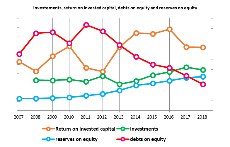
4           Conclusions: a chart to summarize

As to draw a brief concluding summary, it is proposed a graphic summary of the elements that seem to characterize the progress of this sample in the past twelve years, seven of which, in the company of the MTI.

After defining and analysing many tables and as many graphs,  in this research the reader came across a chart that summarized, according to the author, the most important elements that had characterized the economy of a country over time. What was striking was the ability to synthesize a multiplicity of different aspects even in the value scales.  Hence the idea of proposing a summary which, by using some of the indicators, proposed a unitary graphic representation.

The original indicators have different size scales; therefore, in order to allow their representation in a single graph, they all fell back on a single scale from 0 to 100. The indicators are: return on invested capital as a measure of profitability, investments per inhabitant as a measure of investments made, reserves on equity as an indicator of the capitalization of companies and finally, debts in relation to equity, as an indicator of debt. Is it possible to read the graph from a chosen variable by starting from return on investment (RCI) whose growth evidently starts with MTI. This allowed the growth of investments yet, at the same time, allowed the growth of reserves while the debt falls. The conclusion is always the same: if profitability allows investments to grow and companies capitalize a large part of this profitability, yet indebtedness decreases well below what is considered investment grade, then this implies that there is a part of the leverage that is not being used and therefore investments are below of what could have been achieved.

References

AEEG. (2012). Regolazione dei servizi idrici: approvazione del metodo tariffario transitorio (MTT) per la determinazione delle tariffe negli anni 2012 e 2013 – Deliberazione 28 dicembre 2012 585/2012/R/ID. Milano: Autorità per l’energia elettrica e il gas.

AEEGSI. (2013). Delibera 643/2013/R/idr “Approvazione del metodo tariffario idrico e delle disposizioni di completamento “. Milano: Autorità per l’Energia Elettrica e il Gas.

AEEGSI. (2015). Delibera 664/2015/R/idr “Approvazione del metodo tariffario idrico per il secondo periodo regolatorio MTI-2”. Milano: Autorità per l’Energia Elettrica e il Gas.

AEEGSI. (2017). Relazione annuale sullo stato dei servizi e sull’attività svolta (Vol. I Stato dei servizi). Milano: Autorità per l’energia elettrica, il gas e il sistema idrico.

AEEGSI. (2017a). Delibera 918/2017/R/idr “Aggiornamento biennale delle predisposizioni tariffarie del servizio idrico integrato”. Milano: Autorità per l’Energia Elettrica il Gas e il Sistema Idrico.

AEEGSI. (2017b). Delibera 917/2017/R/idr “Regolazione della qualità tecnica del servizio idrico integrato ovvero di ciascuno dei singoli servizi che lo compongono (RQTI)”. Milano: Autorità per l’Energia Elettrica il Gas e il Sistema Idrico.

AEEGSI. (2017c). Delibera 897/2017/R/idr “Approvazione del testo integrato delle modalità applicative del bonus sociale idrico per la fornitura di acqua agli utenti domestici economicamente disagiati”. Milano: Autorità per l’Energia Elettrica il Gas e il Sistema Idrico.

Banca d’Italia, B. (2019). Base dati statistica. Tratto il giorno novembre 11, 2019 da https://infostat.bancaditalia.it: https://infostat.bancaditalia.it/inquiry/#eNqdzs0KwjAQBOAXCttELSWFHGy6hYUmliYV8VJ6qCIULET8AR%2Fe4Klehb18w8DsbXhec90V6NCr%0ApiWre7Jlz%2Fl7AbHE6gfxGHk0Dms8qmJrekMtGBBrzrngEJVuhAAJMuUgYgiuoCwD7FoQsSBlxnYN%0AWnUapjAm45zXWpFnaPeqpj0y7Q%2BqpKpKwvw6T0MIyf0yPr4%2

Bayliss, K., & Hall, D. (2017, May). Bringing water into public ownership: costs and benefints.

Canitano, G., & Peruzzi, P. (2018). L’impatto della regolazione tariffaria sugli investimenti nei servizi idrici. Una ricerca sulle tendenze negli ultimi dieci anni (2007-2016). .NET(61).

Canitano, G., Peruzzi, P., & Todini, L. (2016, ottobre-dicembre). La regolazione tariffaria del Servizio Idrico Integrato in Italia alla luce della teoria e delle esperienze di regolazione incentivante. Management delle infrastrutture e delle utilities(4).

(s.d.). D.M. 1 agosto 1996 “Metodo normalizzato per definire le componenti di costo e determinare la tariffa di riferimento”.

European Central Bank – StatisticalDataWarehouse. (2019). Italy, Long-term interest rate for convergence purposes – Unspecified rate type, Debt security issued, 10 years maturity, New business coverage, denominated in Euro – Unspecified counterpart sector. Tratto il giorno novembre 11, 2019 da https://sdw.ecb.europa.eu: https://sdw.ecb.europa.eu/quickview.do?SERIES_KEY=229.IRS.M.IT.L.L40.CI.0000.EUR.N.Z

EuropeEconomics. (2009). Cost of Capital and Financeability at PR09. Updated Report by Europe Economics. London: Europe Economics.

Green, R., & Pardina, M. R. (1999). Resetting price controls for privatized utilities : a manual for regulators. World Bank Institute (WBI). Washington, DC: World Bank.

OFWAT. (2011, march). Financeability and financing the asset base – A discussion paper. Birmingam: OFWAT.

Utilitatis. (2017). BlueBook. I dati sul Servizio Idrico Integrato in Italia. Roma: Fondazione Utilitatis pro aqua energia ambiente.

Utilitatis. (2019). Blue Book. I dati sul servizio idrico integrato in Italia. Roma: Utilitatis. Pro acqua energia ambiente.

[1] (D.M. 1 agosto 1996 “Metodo normalizzato per definire le componenti di costo e determinare la tariffa di riferimento”)